Analysis in R: 44 color palettes “colormap” package

公開日 2023-02-04

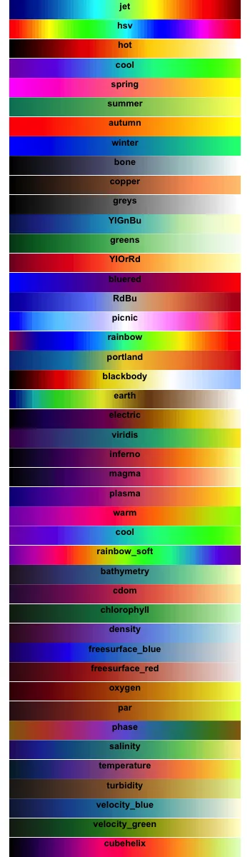
This is an introduction to a package that contains 44 color palettes. It is an easy to use palette.

The included color palette is introduce in the run command and rmd file. Run the “install package” command before running the program. Note that it is recommended to run the program in RStudio.

The package version is 0.1.4. The executable command is RStudio Desktop 2021.09.2+382, R version 4.2.2.

＜おすすめのRに関する書籍です＞

超入門! Rでできるビジュアル統計学学会・論文発表に役立つデータ可視化マニュアル

学会発表や論文の図表づくりに寄せた実践書。伝わるグラフをRで作るための手順をまとめている。

www.amazon.co.jp

Install Package

Run the following command.

#Install Package
install.packages("colormap")
install.packages("tidyverse")
install.packages("flexdashboard")
install.packages("DT")

Example

Check the command, Rmd file (encoding: UTF-8), and package help for details。

Rmd file：colormap ダウンロード

---
title: "colormap package"
output:
  flexdashboard::flex_dashboard:
    orientation: columns
    social: menu
    source_code: embed
runtime: shiny
---

```{r global, include=FALSE}
#Loading Libraries
library("colormap")
library("tidyverse")
library("flexdashboard")
library("DT")

###Create Data#####
n <- 100
TestData <- data.frame("Group" = sample(paste0("Group", 1:5), n, replace = TRUE),
                       "Data1" = sample(1:10, n, replace = TRUE),
                       "Data2" = sample(LETTERS[1:24], n, replace = TRUE))
########
#「colormap」package:Color palette Name：
GgSColName <- c("jet","hsv","hot","cool","spring","summer",
                "autumn","winter","bone","copper","greys",
                "YIGnBu","greens","YIOrRd","bluered","RdBu",
                "picnic","rainbow","portland","blackbody","earth",
                "electric","viridis","inferno","magma","plasma",
                "warm","cool","rainbow-soft","bathymetry","cdom",
                "chlorophyll","density","freesurface-blue","freesurface-red",
                "oxygen","par","phase","salinity","temperature","turbidity",
                "velocity-blue","velocity-green","cubehelix")
```

Column {data-width=500}
-------------------------------------
```{r}
selectInput('Colpal', 'Select Color Palette Name', GgSColName)
sliderInput('ColNo', 'Select No：', value = 5, min = 5, max = 20)

```

###Contains 44 color palettes:

```{r}
renderDataTable({
 ColCodeData <- data.frame("Color_Code" = as.character(colormap_pal(colormap = input$Colpal)(input$ColNo)),
                           "Color" = "")
  datatable(ColCodeData, rownames = FALSE,
            options = list(pageLength = 10, lengthMenu = c(20, 40, 100))) %>%
    formatStyle("Color", valueColumns = "Color_Code",
                backgroundColor = styleEqual(ColCodeData[, 1], ColCodeData[, 1]))
})
```

Column {data-width=500}
-------------------------------------

###ggplot2:color
```{r}
renderPlot({
  ggplot(TestData,
         aes(x = Data1, y = Data2, col = Group)) +
    geom_point(size = 10) +
    theme_bw() +
    scale_color_manual(values = colormap_pal(colormap = input$Colpal)(input$ColNo)) +
    labs(title = paste0("Palette Name：", input$Colpal))
})
```

###ggplot2:fill
```{r}
renderPlot({
  ggplot(TestData,
         aes(x = Data2, fill = Group)) +
    geom_bar(stat = "count") + theme_bw() +
    scale_fill_manual(values = colormap_pal(colormap = input$Colpal)(input$ColNo)) +
    labs(title = paste0("Palette Name：", input$Colpal))
})
```

Supplement

#Show color palettes:colormap command
par(mfrow = c(44,1))
par(mar = rep(0.01, 4))
for(i in seq(colormaps)) {
  barplot(rep(1, 72), yaxt = "n", space = c(0, 0), border = NA,
          col = colormap(colormap = colormaps[[i]]), main = sprintf("\n%s", names(colormaps[i])))
}